Mapping out Trajectories of Charged Defects
Rodrick Kuate Defo, Richard Wang
Professor Manju Manjunathaiah
Introduction
The promise of the nitrogen-vacancy (NV) center in diamond as a system for implementing memory storage for a quantum computer has spawned interest in defect centers in related materials such as SiC. SiC is particularly interesting as it is a polymorphic material, exhibiting about 250 known polytypes, which imbues it with a degree of freedom unavailable in diamond.
The three most common polytypes, 4H- and 6H-SiC and 3C-SiC, all have defects with spin relaxation times ranging from 8 to 24 ms at 20 K (with 4H-SiC being the highest) and coherence persists up to room temperature[1]. In addition to the long spin coherence, a key feature is the ability to optically address (write in and read out) the spin states. However, much of the luminescence or emission of the defects is diverted into transitions involving scattering processes (and is not purely from the desired spin transitions) at ambient temperatures. Indeed, only about 1% of luminescence is from the desired transitions[2].
A potential solution is to place the defects near cavities on resonance with the desired transitions[3]. Positioning defects, however, is a non-trivial endeavor. The defects would be created at roughly the desired location using the process of focused ion beam implantation, but this process creates a lot of damage. In order to heal the damage the sample is annealed, causing the defects to diffuse and some to be lost through conversion to other species. The purpose of this study is then to assess the probability that the negatively charged silicon vacancy defect in 4H-SiC would be optimally positioned and exist given a certain initial position and a certain number of time steps.In Short... We can fire beams at a crystal and create holes in it and if we heal the crystal by heating and cooling, some of these holes move. In diamond, analogous kinds of holes have the potential to be used as a quantum storage device. By modelling this movement in SiC, we can gain insight into memory storage for a quantum computer!
Background
Work has already been done on obtaining barriers to diffusion and the vibrational frequencies that provide the directionality and time scale for the motion[4, 5], but these studies lack a comprehensive understanding of the potential diffusion pathways and as a result do not perform the kinetic Monte Carlo simulations necessary to truly establish diffusion pathways and probabilities with the Coulomb interaction.
Computational Methods
There are two main stages to the calculation of the trajectory probability maps. In the first stage, density functional theory calculations will be carried out to obtain the barriers to diffusion for the various pathways and in the second stage kinetic Monte Carlo simulations will be carried out to map out trajectories. We have existing code for the second part in Matlab, which will be converted to C code. The kinetic Monte Carlo simulations will be carried out with Coulomb interaction and for 1D and 2D random walk test cases (to be compared with theoretical calculations). Without the Coulomb interaction the probability map will be calculated using a breadth first search down the tree of possible transitions (which is $O(log(N))$, where $N$ is the number of possible pathways).
We introduce new notation here. Let $p_{N}(w, x, y, z)$ represent the probability of taking $w$ steps to the right, $x$ steps to the left, $y$ steps upward, and $z$ steps downward, where $w + x + y + z = N$. If some parameters are unwritten, it is assumed that they are $0$. So, $p_{N}(1, 1) = p_{N}(1, 1, 0, 0)$. Similarly, let $P_{N}(x, y)$ be the probability of ending up in position $x$ on the horizontal axis and position $y$ on the vertical axis after $N$ steps. Again, if one of the parameters is unwritten, it is assumed to be zero.
For the 1D case, we let $n_{1}$ be the number of steps to the right and $n_{2}$ be the number of steps to the left. The final position (with rightwards being positive) is then given by $d = n_{1} - n_{2}$ and the total number of steps is $N = n_{1} + n_{2}$. We know that the probability of taking $n_{1}$ steps to the right out of a total of $N$ steps is simply given by the number of ways to permute all the steps divided by the product of the number of ways to permute the right steps and the left steps and multiplied by the probability of taking a right step to the power of $n_{1}$ and the probability of taking a left step to the power of $n_{2}$, so: $$p_{N}(n_{1}, n_{2}) = \left(\frac{1}{2}\right)^{n_{1} + n_{2}}\frac{N!}{n_{1}!n_{2}!} = \left(\frac{1}{2}\right)^{N}\frac{N!}{n_{1}!n_{2}!} = \left(\frac{1}{2}\right)^{N}\frac{N!}{n_{1}!(N-n_{1})!} = \left(\frac{1}{2}\right)^{N}\binom{N}{n_{1}}$$ where we have assumed the probabilities of taking left and right steps to be equal. We can uniquely express $n_{1}$ and $n_{2}$ in terms of $d$ and $N$ by solving the system of two equations, and in doing so we obtain: $$n_{1} = \frac{N+d}{2}, n_{2} = \frac{N-d}{2}$$ Thus, the probability of ending up at a position $d$ after $N$ total steps is simply: $$P_{N}(d) = p_{N}(n_{1}, n_{2}) = \left(\frac{1}{2}\right)^{N}\binom{N}{\frac{N+d}{2}}$$
For the 2D case, we let $n_{1}$ be the number of steps to the right, $n_{2}$ be the number of steps to the left, $n_{3}$ be the number of steps upwards, and $n_{4}$ to be the number of steps downwards. Then: $$p_{N}(n_{1}, n_{2}, n_{3}, n_{4}) = \left(\frac{1}{4}\right)^{N}\frac{N!}{n_{1}!n_{2}!n_{3}!n_{4}!}$$ assuming that the probability of taking a step in any direction is the same. If we let $d_{x} = n_{1} - n_{2}$ be our final horizontal position and $d_{y} = n_{3} - n_{4}$ be the final vertical position, then we can solve for $n_{1}$, $n_{2}$, and $n_{3}$ in terms of $d_{x}, d_{y}, N$, and $n_{4}$: $$n_{1} = \frac{N + d_{x} - d_{y} - 2n_{4}}{2}$$ $$n_{2} = \frac{N - d_{x} - d_{y} - 2n_{4}}{2}$$ $$n_{3} = d_{y} + n_{4}$$ We note that $n_{4}$ can range from $0$ to $\frac{N-d_{x}-d_{y}}{2}$ (the formula holds for $d_{x}, d_{y} \geq 0$ and for negative values of these variables we get infinite denominators for the unnecessary terms from taking factorials of negative numbers so that these unnecessary terms evaluate to zero and it is straightforward to show the expression reduces to the expression with non-negative $d_{x}$, $d_{y}$), so: $$P_{N}(d_{x}, d_{y}) = \sum\limits_{n_{4} = 0}^{\frac{N-d_{x}-d_{y}}{2}} \left(\frac{1}{4}\right)^{N} \frac{N!}{\left(\frac{N+d_{x}-d_{y}-2n_{4}}{2}\right)!\left(\frac{N-d_{x}-d_{y}-2n_{4}}{2}\right)!(d_{y}+n_{4})!n_{4}!}$$ $$= \left(\frac{1}{4}\right)^{N} \frac{\Gamma(N+1) _{2}\tilde{F}_{1}\left(\frac{d_{y}-d_{x}-N}{2}, \frac{d_{x}+d_{y}-N}{2}; 1+d_{y}; 1\right)}{\Gamma\left(\frac{N+2-d_{x}-d_{y}}{2}\right)\Gamma\left(\frac{N+2+d_{x}-d_{y}}{2}\right)}$$ where $\Gamma$ is the gamma function and $_{2}\tilde{F}_{1}$ is the regularized version of the hypergeometric function $_{2}F_{1}$.
Problem Solution
We require multiple pre-determined constants (such as those for transition rates, distances in the lattice cell) before beginning our calculations. Once we have those constants initialized, we can begin work. Transitions in the lattice can go 1 of 12 ways - there are 3 possible transitions out of plane in the upwards direction, 3 possible transitions out of plane in the downwards direction, and 6 possible transitions in the plane. At any given time step, any one of these transitions is possible (with varying probabilities), so the problem (at first pass) grows as $12^N$, where $N$ is the number of time steps. More precisely, positions in 3 dimensions must be computed at each time step, the time must be updated and the probability must be updated for a total of 5 computations for each of the 12 transitions, we must then communicate the results of these 5 computations to the next processor, which will use the calculated values as inputs for an additional 5 units of work for every 12 transitions. Summing the geometric sequence corresponding to the total number of transitions at $0, 1, ... , N$ time steps, we obtain $\frac{12^{N+1}-1}{11}$, so we are dealing with a problem of size $10\cdot \frac{12^{N+1}-1}{11}$, yielding a computational complexity of $O(12^{N+1})$. We use a set of rotation matrices as a simplification in order to calculate movement in any of the in-plane and out of plane directions. Essentially, any given in-plane transition of the six, treating the current position as the origin, can be mapped onto any other in-plane transition of the six by simply rotating the original transition, in-plane, by some multiple of 60 degrees. Similarly, any upwards (downwards) transition can be mapped onto any other upwards (downwards) transition of the three by simply rotating the original transition by some multiple of 120 degrees. Thus, we define three transitions (one in-plane and two out of the plane) and obtain the remaining transitions by using rotation matrices.
Past this point, we fill a matrix $\texttt{A}$ with values corresponding to the $x$, $y$ and $z$ position shifts for a particular transition, the probability of transitioning, and the time shift for the particular transition. From here, we run a breadth-first search (BFS) through the tree with each node corresponding to a particular sequence of transitions, with corresponding particular final $x$, $y$ and $z$ positions and a given final or total time up to that point and a given final or total probability up to that point. There are $N$ layers to this tree and each layer has $12^N$ nodes (for a total of $\frac{12^{N+1}-1}{11}$ nodes in the tree).
Finally, we print out the $x, y, z$ coordinates, the probability of transitioning to that a given location, and the time passed.
Parallelization of BFS
We initially used a recursive crawling method for performing the breadth-first search (BFS) required to map probabilities in the lattice. This method involved traversing to a particular position in the lattice and directly running our BFS function from that position (a recursive call). We found that applying OpenMP directives to the recursive portion was difficult, especially since the probability that a defect appeared in a particular position on the lattice likely depended on other probabilities which may not have been updated.
Instead, we aimed to change the model of how we traverse through the 12-ary tree. We were considering switching entirely to the matrix-vector multiplication method of BFS with the boolean semiring model, but instead we opted for a serial traversal of BFS that still adopted the semiring model. We use two different semirings - one for updating the probability and one for updating the position and time steps. This semiring model is described in more detail in the advanced features section. This made it easier for us to directly write parallelizing pragmas because our serial implementation resulted in several $\texttt{for}$ loops which are simple to parallelize.
The .gifs were obtained by calculating the probability map for a system size of $\frac{12^{6}-1}{11}$ different pathways. Figure II shows the preprocessed data for the transitions that were calculated. Figures III and IV show the same data, except averaged over the two types of transitions.
SPMD shared memory with OpenMP
We used the SPMD paradigm of parallelism in order to achieve initial speedup. We used the standard library for shared memory multiprocessing, OpenMP. When parallelizing $\texttt{for}$ loops, we used the standard compiler directive $\texttt{pragma omp parallel}$, designating shared matrices and iterators appropriately with the $\texttt{shared}$ and $\texttt{private}$ keywords.
Initially, we tried applying OpenMP pragmas to every easily parallelizable section of the code. We realized this created too much parallel overhead, since a lot of the operations we aimed to parallelize involved $3 \times 3$ matrices (matrix-matrix multiplication, vector-matrix multiplication, etc.), and the cost of starting up threads comparing to the speedup from distributing the work simply was not worth it.
With the serial implementation of BFS in place, we were simply able to apply an OpenMP pragma to a loop in order to quickly iterate through the particles in the lattice. Additionally, we were able to quickly iterate through printing the probabilities of transitioning to positions by parallelizing that portion (this was especially simple since we don't care about the order in which we print things after they are calculated!).
Hybrid SPMD with OpenMP-MPI
We used the common hybrid model of combining message passing with MPI with OpenMP. By splitting the work that needs to be done across several nodes, we can achieve further speedup.
In our particular usage of MPI, we use $\texttt{MPI_Isend}$ calls with the $\texttt{swtcher}$ variable to communicate to a node that calculations corresponding to a particular transition (as determined by the $\texttt{swtcher}$ variable) needs to be done.
Once all of the calculations are done, if we are in the root process, we print out the probabilities of transitioning to a particular location.
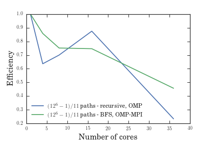
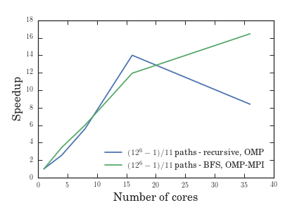
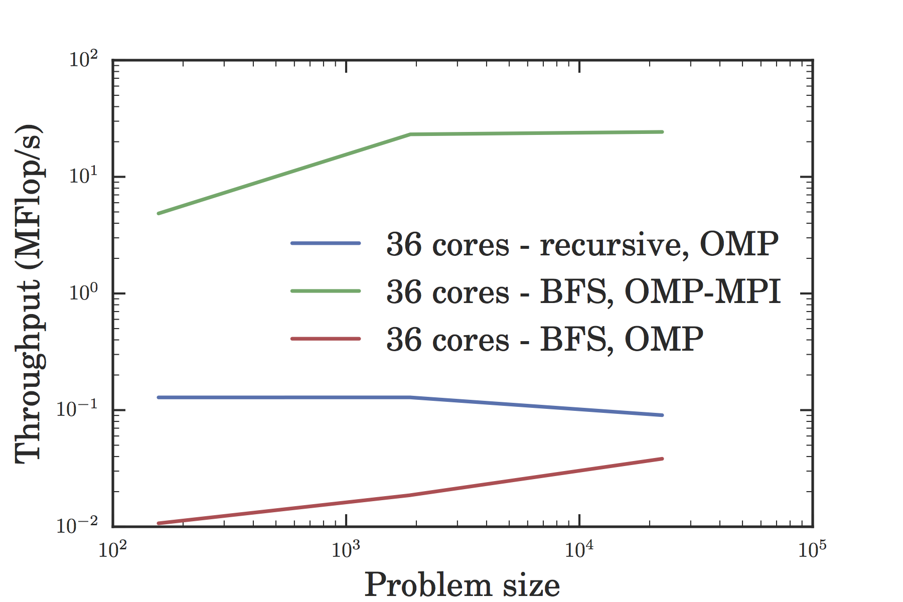
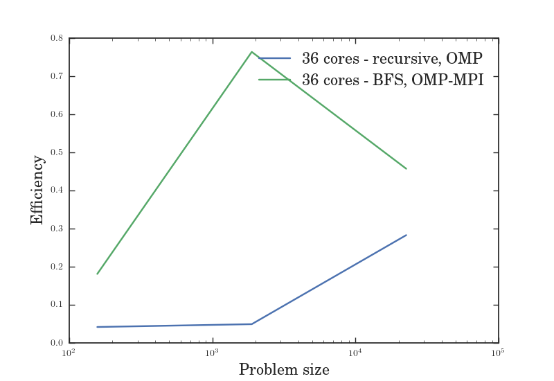
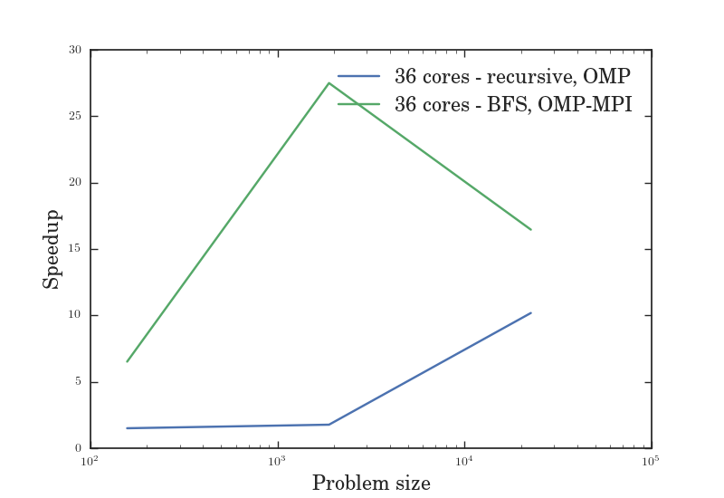
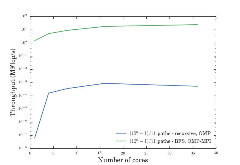
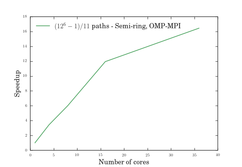
As we can see from Figure VII, the serial BFS solution might have been slower than the recursive solution, but the serial approach to BFS made it easier for us to utilize the hybrid OpenMP-MPI model which led to greater speedup. Figures V through VII give us the efficiency, speedup, and throughput for a variable number of cores given a fixed problem size, while figures VIII through X give us the efficiency, speedup, and throughput for a fixed number of cores given a variable problem size. In all of these graphs, the OMP-MPI hybrid solution is seen to be around as good as, if not far outperforming, the OpenMP solution.
Advanced features
Semiring model
One of the advanced features we used was to convert our initially recursive implementation of BFS to a model similar to the semiring model. The initial, immediate advantage to this was that we could convert a recursive implementation into a serial one, which is an advantage in the ease of parallelization.
A disclaimer is that we cannot use the pure boolean semiring $(\{0, 1\}, |, \&)$. The reason for this is that the boolean semiring is used for determining whether or not we are able to traverse to a particular node in BFS. We care about more than that - we care about the probability of transition to a certain point, the coordinates associated with those points, and the time steps required to reach those points. Because of this, using a pure semiring is not feasible.
However, there are several important takeaways from the boolean semiring model that we can use to construct our own implementation of BFS. One of them is that we can use a semiring - the semiring of $([0, \infty], +, \times)$, which will generally cover the cases we require for our lattice traversal. Another very important idea is the construction of a graph as a matrix. Initially, we were considering tree traversal in a context conducive to human understanding - traversing down a branch of the tree. But by converting our tree to a matrix representation, we were able to gain insight on how to construct a serial implementation of BFS and therefore parallelize this operation.
Kinetic Monte Carlo
The naive BFS traversal does not take into account the particle-particle Coulomb interactions that may be occurring as a defect moves through the lattice. In order to take into account this process, we use a simulation called kinetic Monte Carlo, which simulates some process with known transition rates as evolving through time. We need to map out all transitions and obtain their rates. Then, we construct a cumulative vector of transition rates. We choose a random number between 0 and 1 and multiply by the sum of the transition rates, and choose the transition corresponding to the element of the cumulative vector mapped to by this multiplication. Then we update time and restart the process at the new position. This is analogous to the following update to the naive method of finding transition rates:
$$r = \nu\exp\left(-\frac{E_{act}}{k_{B}T}\right) \rightarrow \nu\exp\left(-\frac{(E_{act} + \Delta\phi(\vec{r}))}{k_{B}T}\right)$$
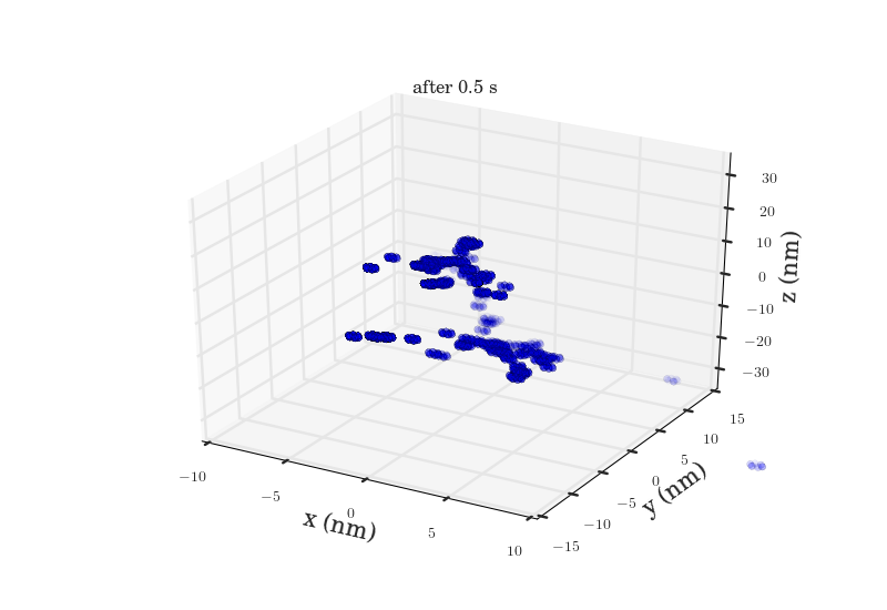
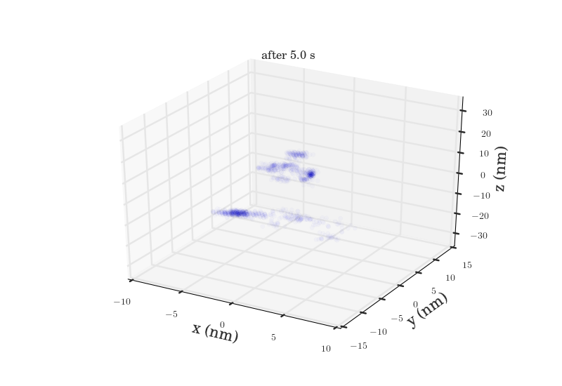
The plots above show the probability map of the vacancies constructed using the kinetic Monte Carlo simulation after 0.5s and 5s. The intensity of the spots correspond to the probability that a vacancy will appear in that spot.
References
- [1] A. L. Falk, B. B. Buckley, G. Calusine, W. F. Koehl, V. V. Dobrovitski, A. Politi, C. A. Zorman, P. X. L. Feng, and D. D. Awschalom, "Polytype control of spin qubits in silicon carbide," Nature Communications, vol. 4, p. 1819, 05 2013.
- [2] I. Aharonovich, S. Castelletto, D. A. Simpson, C.-H. Su, A. D. Greentree, and S. Prawer, "Diamond-based single-photon emitters," Reports on Progress in Physics, vol. 74, no. 7, p. 076501, 2011.
- [3] D. O. Bracher, X. Zhang, and E. L. Hu, "Selective purcell enhancement of two closely linked zero-phonon transitions of a silicon carbide color center," arXiv:1609.03918, 2016.
- [4] E. Rauls, T. Frauenheim, A. Gali, and P. Deák, "Theoretical study of vacancy diffusion and vacancy-assisted clustering of antisites in sic," Phys. Rev. B, vol. 68, p. 155208, Oct 2003.
- [5] X. Wang, M. Zhao, H. Bu, H. Zhang, X. He, and A. Wang, "Formation and annealing behaviors of qubit centers in 4h-sic from first principles," Journal of Applied Physics, vol. 114, no. 19, p. 194305, 2013.